Zipf's law
ests.visualizers.zipf(), ests.visualizers.zipf_theory()
Description
Plotting Zipf's law from a counter of the frequencies of words.
Definition
Zipf's law (the rank-frequency law) is an empirical regularity of the distribution of the frequencies of words in a natural language: if all the words of a language, or of a long enough text, are ordered by descending frequency, the frequency of the n-th word of the list is roughly inversely proportional to its number n, the rank of the word. The second most frequent word occurs about half as often as the first, the third a third as often, and so on.
Parameters
| Parameter | Type | Default | Description |
|---|---|---|---|
counter |
Counter | - |
Counter of the frequencies of words |
num_words |
int | None |
Number of the most frequent words |
num_labels |
int | 10 |
Number of the words labelled on the plot |
log |
bool | True |
Use a logarithmic scale |
show_theory |
bool | False |
Plot the theoretical Zipf's law |
alpha |
float | 1.5 |
Exponent α of the theoretical Zipf's law, greater than zero |
show_fit |
bool | False |
Plot the Zipf-Mandelbrot fit \(f(r) = C / (r + q)^s\) of fit_zipf_mandelbrot |
ax |
Axes | None |
Axes of matplotlib for the plot; if not given, a new figure is created |
The function returns the Axes with the plot; a num_words greater than the number of word types does not extend the curves beyond the data, and an empty counter raises SourceError. zipf_theory(size, num_ranks, alpha, ax) plots the theoretical curve alone, \(f(r) = size \cdot r^{-\alpha}\) for the ranks from 1 to num_ranks.
Usage example
The lemmas of Marianela by Galdós from Project Gutenberg.
Example
Code:
from collections import Counter
from urllib.request import urlopen

from ests import WordsExtractor
from ests.visualizers import zipf

url = "https://www.gutenberg.org/cache/epub/17340/pg17340.txt"
text = urlopen(url).read().decode("utf-8")
text = text[text.index("\n", text.index("*** START OF")) : text.index("*** END OF")]
counts = Counter(WordsExtractor(use_lexemes=True, lowercase=True, filter_nums=True).extract(text))

ax = zipf(counts, num_labels=10, show_theory=True, alpha=1.0, show_fit=True)
ax.figure.savefig("zipf.png")
Result:
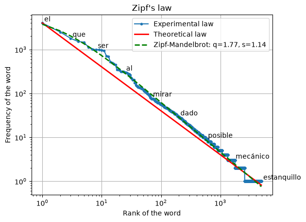
On logarithmic axes the frequencies of the lemmas fall along a straight line; the Zipf-Mandelbrot fit, \(s = 1.14\) with a shift \(q = 1.77\), follows them closer than the theoretical law with \(\alpha = 1\) at the head of the list.