Vocabulary growth and frequency spectrum¶

ruts.visualizers.heaps_plot(), ruts.visualizers.frequency_spectrum_plot()

Description¶

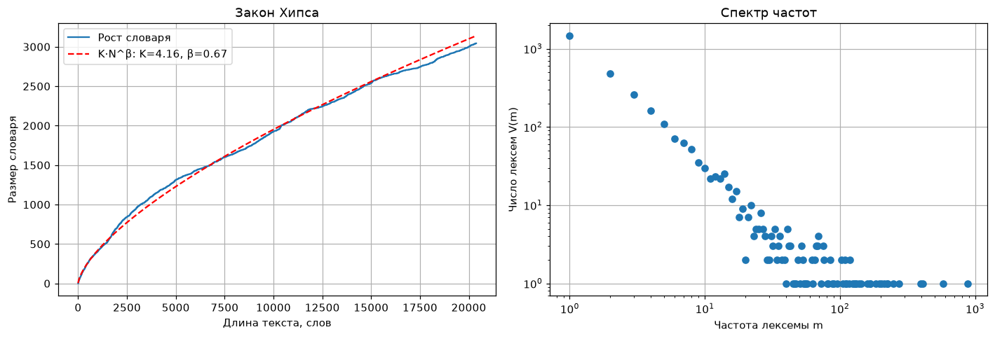
Two plots about the word distribution of a text complementing Zipf's law: vocabulary growth with text length by Heaps' law and the frequency spectrum - how many lexemes occur exactly once, twice, three times. Both plots exist in zipfR (plot.vgc, plot.spc). The functions take axes ax and return Axes.

Heaps' law¶

The vocabulary size \(V\) after every word of the text and the fitted curve \(V(N) = K \cdot N^{\beta}\) by fit_heaps with the parameters in the legend. On corpora of millions of words \(\beta\) lies within 0.4-0.6; over the whole growth curve of a single text it comes out higher (0.6-0.9), since at the beginning of a text almost every word is new; the curve depends on word order.

Parameter	Type	Default	Description
`words`	list[str]	`-`	Words of the text in order
`ax`	Axes	`None`	Axes for the plot

Frequency spectrum¶

The number of lexemes \(V(m)\) occurring exactly \(m\) times (calc_frequency_spectrum) in logarithmic coordinates; the left edge is the hapaxes. The spectrum underlies the diversity measures of Yule, Sichel, Michéa and Honoré, and its shape shows how "undersampled" the vocabulary of the text is.

Parameter	Type	Default	Description
`words`	list[str]	`-`	Words of the text
`ax`	Axes	`None`	Axes for the plot

Usage example¶

Example

Code:

# Import the libraries
import matplotlib.pyplot as plt
from ruts import WordsExtractor
from ruts.datasets import StalinWorks
from ruts.visualizers import frequency_spectrum_plot, heaps_plot

# Prepare the data
sw = StalinWorks()
we = WordsExtractor(use_lexemes=True, lowercase=True, filter_nums=True)
lemmas = [lemma for text in sw.get_texts(limit=12) for lemma in we.extract(text)]

# Plot
fig, (left, right) = plt.subplots(1, 2, figsize=(13, 4.5))
heaps_plot(lemmas, ax=left)
frequency_spectrum_plot(lemmas, ax=right)

Result:

ruts